This is a first post of the Deep Learning for Computer Vision (DL4CV) tutorial series. For different types of the computer vision problems, deep learning techniques have achieved high accuracy. Image classification is a well defined problem in image processing and computer vision. We are going to perform image classification using a well known deep learning technique - CNN (Convolutional Neural Network). The CNNs are very useful for to perform image processing and computer vision related tasks efficiently. We will use CIFAR 10 dataset for training and testing the CNN model. Let's take a deep dive into the steps to understand how the image classification works. In this project, we will cover the following topics.
Table of Contents:
- Prerequisites
- Import Required Libraries
- Load CIFAR10 Dataset
- Visualize Random Images from the Dataset
- Define a Convolutional Neural Network (CNN)
- Define a Loss Function and an Optimizer
- Train the Network on the training data
- Test/ Evaluate the Network on Test Data
Prerequisites
- Language: Python 3 or Higher
- Frameworks: TensorFlow
- Libraries: NumPy, Matplotlib and scikit-learn
Import Required Libraries
Now we import all the required libraries and framework.
import tensorflow as tfWe import tensorflow as tf. Also the image datasets, CNN layers and models are imported from tensorflow.keras. Here Keras is a deep learning API written is Python. We different scikit-learn metrics from sklearn.metrics. The libraries Matplotlib and NumPy also imported as well.
from tensorflow.keras import datasets, layers, models
import matplotlib.pyplot as plt
from sklearn.metrics import confusion_matrix , classification_report
import numpy as np
Load CIFAR10 dataset
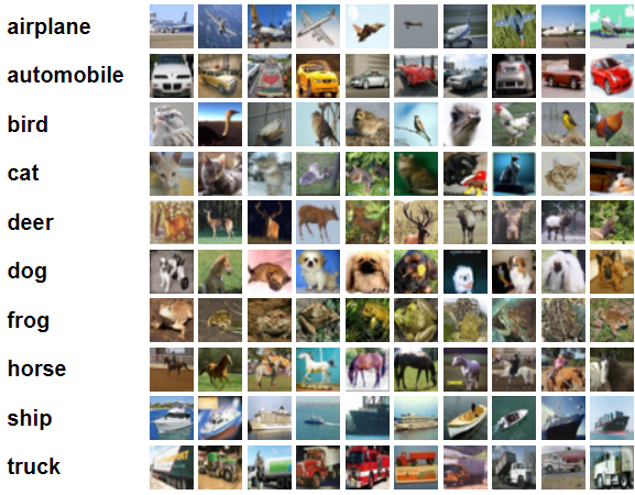
After importing the required libraries and frameworks, the next task is to load the CIFAR 10 dataset.["airplane","automobile","bird","cat","deer","dog","frog","horse","ship","truck"]
 |
| CIFAR-10 Images with 10 Classes Image Source: https://www.cs.toronto.edu/~kriz/cifar.html |
(X_train, y_train), (X_test, y_test) = datasets.cifar10.load_data()
X_train.shape
Output
Downloading data from https://www.cs.toronto.edu/~kriz/cifar-10-python.tar.gzYou can notice that the total images in the train dataset is 50,000. The size of each image is (32,32,3). The image height and width is 32 each having 3 channels- RGB.
170500096/170498071 [==============================] - 3s 0us/step
170508288/170498071 [==============================] - 3s 0us/step
(50000, 32, 32, 3)
X_test.shape
(10000, 32, 32, 3)There are 10,000 images in test dataset each having the size of (32,32,3) as the same train dataset.
y_train.shape
(50000, 1)
y_test.shape
(10000, 1)
To learn more about pre-processing of CIFAR-10 dataset please refer to below article.
How to Load, Pre-process and Visualize CIFAR-10 and CIFAR -100 datasets in PythonVisualize Random Images from CIFAR10 Dataset
Now we have loaded the train and test datasets, let's visualize some images to understand how the images from CIFAR 10 datasets look like.class_names = ['airplane', 'automobile', 'bird', 'cat', 'deer', 'dog', 'frog', 'horse', 'ship', 'truck']
plt.figure(figsize=(10,10))
for i in range(25):
plt.subplot(5,5,i+1)
plt.xticks([])
plt.yticks([])
plt.grid(False)
plt.imshow(train_images[i])
# The CIFAR labels happen to be arrays,
# which is why you need the extra index
plt.xlabel(class_names[train_labels[i][0]])
plt.show()
Output

X_train = X_train / 255.0
X_test = X_test / 255.0
Define a Convolutional Neural Network (CNN)
# number of classes
y_train = y_train.reshape(-1,)
K = len(set(y_train))

# calculate total number of classes
# for output layer
print("number of classes:", K)

# Build the model using the functional API
# input layer
model = models.Sequential()
model.add(layers.Conv2D(32, (3, 3), activation='relu', padding='same', input_shape=(32, 32, 3)))
model.add(layers.BatchNormalization())
model.add(layers.Conv2D(32, (3, 3), activation='relu', padding='same'))
model.add(layers.BatchNormalization())
model.add(layers.MaxPooling2D((2, 2)))
model.add(layers.Conv2D(64, (3, 3), activation='relu', padding='same'))
model.add(layers.BatchNormalization())
model.add(layers.Conv2D(64, (3, 3), activation='relu', padding='same'))
model.add(layers.BatchNormalization())
model.add(layers.MaxPooling2D((2, 2)))
model.add(layers.Conv2D(128, (3, 3), activation='relu', padding='same'))
model.add(layers.BatchNormalization())
model.add(layers.Conv2D(128, (3, 3), activation='relu', padding='same'))
model.add(layers.BatchNormalization())
model.add(layers.MaxPooling2D((2, 2)))
model.add(layers.Flatten())
model.add(layers.Dropout(0.2))

# Hidden layer
model.add(layers.Dense(1024, activation='relu'))
model.add(layers.Dropout(0.2))

# last hidden layer i.e.. output layer
model.add(layers.Dense(K, activation='softmax'))


# model description
model.summary()
Output
number of classes: 10
Model: "sequential"
_________________________________________________________________
 Layer (type)                Output Shape              Param #
=================================================================
 conv2d (Conv2D)             (None, 32, 32, 32)        896

 batch_normalization (BatchN  (None, 32, 32, 32)       128
 ormalization)

 conv2d_1 (Conv2D)           (None, 32, 32, 32)        9248

 batch_normalization_1 (Batc  (None, 32, 32, 32)       128
 hNormalization)

 max_pooling2d (MaxPooling2D  (None, 16, 16, 32)       0
 )

 conv2d_2 (Conv2D)           (None, 16, 16, 64)        18496

 batch_normalization_2 (Batc  (None, 16, 16, 64)       256
 hNormalization)

 conv2d_3 (Conv2D)           (None, 16, 16, 64)        36928

 batch_normalization_3 (Batc  (None, 16, 16, 64)       256
 hNormalization)

 max_pooling2d_1 (MaxPooling  (None, 8, 8, 64)         0
 2D)

 conv2d_4 (Conv2D)           (None, 8, 8, 128)         73856

 batch_normalization_4 (Batc  (None, 8, 8, 128)        512
 hNormalization)

 conv2d_5 (Conv2D)           (None, 8, 8, 128)         147584

 batch_normalization_5 (Batc  (None, 8, 8, 128)        512
 hNormalization)

 max_pooling2d_2 (MaxPooling  (None, 4, 4, 128)        0
 2D)

 flatten (Flatten)           (None, 2048)              0

 dropout (Dropout)           (None, 2048)              0

 dense (Dense)               (None, 1024)              2098176

 dropout_1 (Dropout)         (None, 1024)              0

 dense_1 (Dense)             (None, 10)                10250

=================================================================
Total params: 2,397,226
Trainable params: 2,396,330
Non-trainable params: 896
_________________________________________________________________
Notice total, trainable and non-trainable parameters in the network.Now we defined successfully our CNN model. Let's move to define the loss function and optimizer.
Define a Loss Function And an Optimizer
optimizer = 'adam'
loss = 'sparse_categorical_crossentropy'
Compile the Model
model.compile(optimizer='adam',loss = 'sparse_categorical_crossentropy',metrics=['accuracy'])
Now we have set the loss function and optimizer, we can move to train our network.
Train the Network on Training Data
history = model.fit(X_train, y_train, epochs=20, validation_data=(X_test, y_test))
Output
Epoch 1/20
1563/1563 [==============================] - 42s 21ms/step - loss: 1.3265 - accuracy: 0.5468 - val_loss: 1.0588 - val_accuracy: 0.6208
Epoch 2/20
1563/1563 [==============================] - 32s 21ms/step - loss: 0.8544 - accuracy: 0.7032 - val_loss: 0.8160 - val_accuracy: 0.7154
Epoch 3/20
1563/1563 [==============================] - 30s 19ms/step - loss: 0.6999 - accuracy: 0.7583 - val_loss: 0.7447 - val_accuracy: 0.7468
Epoch 4/20
1563/1563 [==============================] - 31s 20ms/step - loss: 0.5927 - accuracy: 0.7961 - val_loss: 0.8862 - val_accuracy: 0.7116
Epoch 5/20
1563/1563 [==============================] - 32s 20ms/step - loss: 0.5013 - accuracy: 0.8284 - val_loss: 0.6328 - val_accuracy: 0.7899
Epoch 6/20
1563/1563 [==============================] - 32s 21ms/step - loss: 0.4335 - accuracy: 0.8512 - val_loss: 0.7026 - val_accuracy: 0.7836
Epoch 7/20
1563/1563 [==============================] - 32s 21ms/step - loss: 0.3595 - accuracy: 0.8761 - val_loss: 0.6304 - val_accuracy: 0.8020
Epoch 8/20
1563/1563 [==============================] - 32s 21ms/step - loss: 0.3076 - accuracy: 0.8959 - val_loss: 0.6027 - val_accuracy: 0.8092
Epoch 9/20
1563/1563 [==============================] - 33s 21ms/step - loss: 0.2648 - accuracy: 0.9094 - val_loss: 0.6441 - val_accuracy: 0.8167
Epoch 10/20
1563/1563 [==============================] - 43s 28ms/step - loss: 0.2249 - accuracy: 0.9239 - val_loss: 0.6653 - val_accuracy: 0.8067
Epoch 11/20
1563/1563 [==============================] - 33s 21ms/step - loss: 0.1943 - accuracy: 0.9339 - val_loss: 0.6418 - val_accuracy: 0.8145
Epoch 12/20
1563/1563 [==============================] - 44s 28ms/step - loss: 0.1755 - accuracy: 0.9396 - val_loss: 0.6752 - val_accuracy: 0.8246
Epoch 13/20
1563/1563 [==============================] - 35s 23ms/step - loss: 0.1570 - accuracy: 0.9462 - val_loss: 0.6706 - val_accuracy: 0.8325
Epoch 14/20
1563/1563 [==============================] - 42s 27ms/step - loss: 0.1499 - accuracy: 0.9506 - val_loss: 0.7519 - val_accuracy: 0.8210
Epoch 15/20
1563/1563 [==============================] - 33s 21ms/step - loss: 0.1345 - accuracy: 0.9558 - val_loss: 0.6644 - val_accuracy: 0.8235
Epoch 16/20
1563/1563 [==============================] - 32s 21ms/step - loss: 0.1291 - accuracy: 0.9571 - val_loss: 0.8130 - val_accuracy: 0.8080
Epoch 17/20
1563/1563 [==============================] - 33s 21ms/step - loss: 0.1154 - accuracy: 0.9607 - val_loss: 0.7475 - val_accuracy: 0.8273
Epoch 18/20
1563/1563 [==============================] - 33s 21ms/step - loss: 0.1097 - accuracy: 0.9636 - val_loss: 0.7086 - val_accuracy: 0.8355
Epoch 19/20
1563/1563 [==============================] - 31s 20ms/step - loss: 0.1001 - accuracy: 0.9665 - val_loss: 0.7216 - val_accuracy: 0.8355
Epoch 20/20
1563/1563 [==============================] - 30s 19ms/step - loss: 0.1011 - accuracy: 0.9661 - val_loss: 0.7446 - val_accuracy: 0.8364
We train our network for 20 epochs. You can train for hundreds of epochs. Notice the accuracy is increasing slowly for higher epochs.
We get the training accuracy of 96.61% and the validation accuracy of 83.64%.
You may increase these accuracies by training the model for more epochs. You may use use data augmentation also. This also helps achieving better validation accuracy using the technique of data augmentation. Data augmentation is a technique for data pre-processing. Using this technique we generate different types of images by transforming the images available in the dataset.
Here we have completed the training part of the model. Now move to test or evaluate our network/ model.
Test/ Evaluate the Network on Test Data
Now evaluate the model on the test data. Find the predicted scores and classes of test dataset using model.predict(X_test).
y_pred = model.predict(X_test)Let's print the test scores for each class and for all images in the test dataset.
y_pred_classes = [np.argmax(element) for element in y_pred]
y_pred
Output:
  [[3.9521787e-08 2.3015059e-09 4.6826610e-08 ... 1.2385266e-07
  9.0896992e-07 1.3537279e-07]
 [1.9760818e-19 1.0568182e-09 1.0820759e-28 ... 4.4578180e-30
  1.0000000e+00 1.6756009e-20]
 [2.0620810e-05 4.2299676e-04 4.2718745e-11 ... 3.5415070e-08
  9.9945992e-01 1.6858961e-06]
 ...
 [8.3391088e-15 6.5921789e-14 1.1535729e-08 ... 4.8390071e-08
  1.4339907e-13 4.2596921e-13]
 [9.9146479e-01 9.9901354e-04 1.1814365e-03 ... 4.7673228e-05
  5.9958766e-03 1.1494376e-05]
 [1.4169767e-16 7.0683491e-16 2.0917616e-15 ... 1.0000000e+00
  3.8461754e-17 8.3701241e-14]]
y_pred_classes
Output:
["airplane","automobile","bird","cat","deer","dog","frog","horse","ship","truck"]
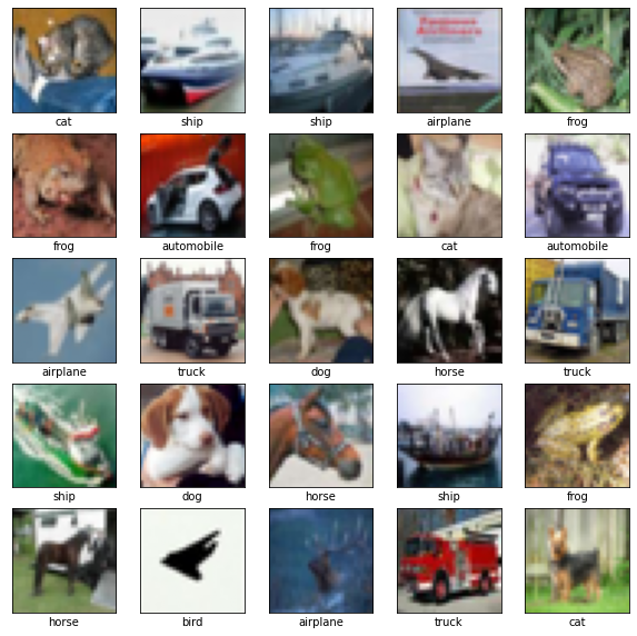
Predict Some Result
labels = ['airplane', 'automobile', 'bird', 'cat', 'deer', 'dog', 'frog', 'horse', 'ship', 'truck']
y_pred = model.predict(X_test)
print(y_pred)
y_classes = [np.argmax(element) for element in y_pred]
//print(y_classes)
plt.figure(figsize=(10,10))
for i in range(25):
     plt.subplot(5,5,i+1)
     plt.xticks([])
     plt.yticks([])
     plt.grid(False)
     plt.imshow(X_test[i])
     # The CIFAR labels happen to be arrays,
     # which is why you need the extra index
     # print(y_train[i])
     # plt.xlabel("True class:{} "'\n Predicted class: {}' ,labels[y_train[i]], )
     plt.xlabel(labels[y_classes[i]])
plt.show()
Ouput
 |
| 25 Images with predicted class labels |
Plot Accuracy
plt.plot(history.history['accuracy'], label='accuracy')
plt.plot(history.history['val_accuracy'], label = 'val_accuracy')
plt.xlabel('Epoch')
plt.ylabel('Accuracy')
plt.ylim([0.7, 1])
plt.legend(loc='lower right')

test_loss, test_acc = model.evaluate(X_test,  y_test, verbose=2)
Output
313/313 - 2s - loss: 0.7446 - accuracy: 0.8364 - 2s/epoch - 7ms/step
 |
| training and validation accuracies |
Analyze the two accuracies- training and validation.
Classification Report
print("Classification Report: \n", classification_report(y_test, y_pred_classes))Output:
Classification Report:
               precision    recall  f1-score   support

           0       0.83      0.88      0.85      1000
           1       0.93      0.93      0.93      1000
           2       0.77      0.76      0.77      1000
           3       0.65      0.73      0.69      1000
           4       0.84      0.80      0.82      1000
           5       0.81      0.75      0.78      1000
           6       0.90      0.85      0.87      1000
           7       0.89      0.85      0.87      1000
           8       0.86      0.93      0.89      1000
           9       0.92      0.89      0.90      1000

    accuracy                           0.84     10000
   macro avg       0.84      0.84      0.84     10000
  weighted avg       0.84      0.84      0.84     10000
Confusion Matrix
print("confusion matrix:\n", confusion_matrix(y_test, y_pred_classes))Output:
confusion matrix:
 [[879   4  31  12   4   4   3   6  44  13]
 [  9 934   2   2   1   1   2   1  18  30]
 [ 48   7 763  53  43  33  26  16   8   3]
 [ 19   6  49 731  33  80  33  23  20   6]
 [ 18   3  55  54 796  18  17  33   6   0]
 [  9   1  27 153  25 747   7  23   4   4]
 [ 11   3  30  50  19  16 846   3  17   5]
 [ 10   1  25  49  22  26   1 855   6   5]
 [ 37  10   7   5   2   1   2   0 926  10]
  [ 21  40   5  16   1   1   0   0  29 887]]
great
ReplyDelete